Linear Regression predicts the value of a dependent variable (y) given one or more independent variables (x₁, x₂, x₃...x_n). In this case, y is continuous - i.e. it can hold any value.

In many real world problems^[1], however, we often want to predict a binary value instead - where y takes on one of two discrete values rather than being continuous. Logistic Regression (aka Binary Classification), converts the linear combination of input features (the x values seen earlier in multiple regression) into probabilities via a sigmoid^[2] function.

In Logistic regression we'll use the Logistic Function to convert the inputs into probabilities.

The Logistic Function

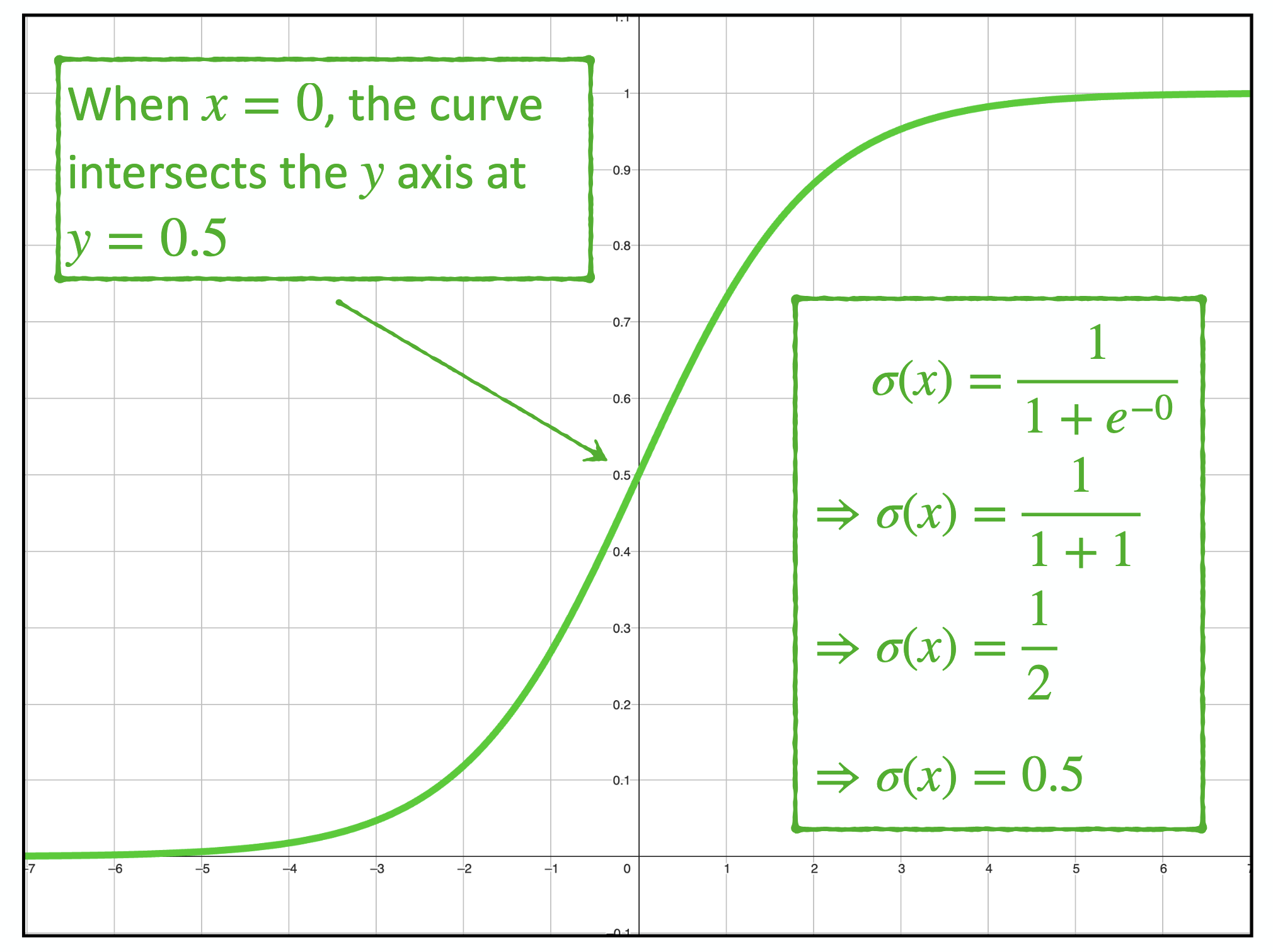
"The logistic function, denoted by the lowercase sigma (σ), is defined as:

This function maps z, to values between 0 and 1 and has the characteristic "S" curve that intersects the Y axis at 0.5

We can then define the predicted value $\hat{y}$ as the sigmoid transformation of the linear combination of parameters:

Representing this in the matrix form gives us:

It is important to note that the vector of observations (X) includes the intercept column (all ones).

With this representation of the model for binary classification, the problem is reduced to finding the optimal values of W, which can be computed using Gradient Descent.

Gradient Descent for Logistic Regression

Gradient descent iteratively minimizes a cost function. For logistic regression, we use the binary cross-entropy cost function:

The first derivative^[3] of the cost function is:

We can now write the gradient descent algorithm in pseudocode as follows:

// Start with initial values for the model coefficients
// W is a k x 1 column vector
W = 0 

for i in 0..iterations:
   // Step 1: compute the predicted values for the model with parameters beta
   // Y_hat is an n x 1 column vector of predictions
   // X is a n x k matrix of feature values
   // W is k x 1 column vector
   Z = matmul(X,W)
   
   // Step 2: Apply the sigmoid
   Y_hat = sigmoid(Z)

   // Step 3: Calculate the error in the predictions
   // Y is an n x 1 column vector of observations
   Y_err = Y_hat - Y
   
   // Step 4: Calculate the first derivative of the cost function (the gradient)
   d_cost = (1/n)matmul(X_transpose, Y_err)
   
   //Step 5: Calculate the step size
   step_size = learning_rate * d_cost
   
   //Step 6: Calculate the new values for the model parameters
   W = W - step_size

The steps for gradient descent (as well as the derivative of the cost function) are the same as those for Multiple Regression with the exception of the sigmoid function.

Logistic Regression in Go

We begin the Go implementation by defining the sigmoid function

func sigmoid(z float64) float64 {
	return 1.0 / (1.0 + math.Exp(-z))
}
 

We also define a struct - LogisticRegression - that holds the training data and the parameters.

type LogisticRegression struct {
	// Column Vector of observed binary labels (0 or 1) (shape: n x 1)
	y *mat.VecDense
	// Matrix of k independent variables and n observations (shape: n x k)
	// First column of x is intercept (all 1.0s)
	x *mat.Dense
	// Number of observations
	n int
	// Number of parameters (features + intercept)
	k int
	// Number of iterations
	iter int
	// learning rate
	lr float64
	// w is the vector of coefficients (includes intercept as w[0])
	w *mat.VecDense
}

func NewLogisticRegression(x *mat.Dense, y *mat.VecDense, iter int, learning_rate float64) *LogisticRegression {
	x_obs, x_vars := x.Dims()
	y_len := y.Len()

	if y_len != x_obs {
		panic("Vector y must be the same length as x.rows")
	}

	// Vector of parameters (k x 1) - includes intercept as w[0]
	// Initialize all weights to 0.0 (including intercept)
	w_init := make([]float64, x_vars)
	for i := range w_init {
		w_init[i] = 0.0
	}

	w := mat.NewVecDense(x_vars, w_init)

	return &LogisticRegression{
		y, x, x_obs, x_vars, iter, learning_rate, w,
	}
}
 

Next we can implement Train() that is used for training the model - we'll use the gonum library for matrix and vector operations.

func (lr *LogisticRegression) Train() {

	// z is the linear combination (n x 1)
	z := mat.NewVecDense(lr.n, make([]float64, lr.n))
	// y_hat is the vector of predicted probabilities 
    // after sigmoid (n x 1)
	y_hat := mat.NewVecDense(lr.n, make([]float64, lr.n))
	// y_err is the error: 
    // diff between predicted probabilities and actual (n x 1)
	y_err := mat.NewVecDense(lr.n, make([]float64, lr.n))
	// dW is the gradient vector (k x 1)
	dW := mat.NewVecDense(lr.k, make([]float64, lr.k))
	// step_size is the update step (k x 1)
	step_size := mat.NewVecDense(lr.k, make([]float64, lr.k))

	// Temporary vector for cost calculation
	cost_vec := mat.NewVecDense(lr.n, make([]float64, lr.n))

	for i := 0; i < lr.iter; i++ {

		// Step 1: Calculate linear combination z = X · W (Shape: n x 1)
		// X includes intercept column, W includes intercept weight
		z.MulVec(lr.x, lr.w)

		// Step 2: Apply sigmoid activation element-wise
		for j := 0; j < lr.n; j++ {
			y_hat.SetVec(j, sigmoid(z.AtVec(j)))
		}

		// Now calculate the derivative w.r.t W 
        // (includes intercept gradient)
		// dW = X^T · (Y_hat - Y) / n

		// Step 3: Calculate y_hat - y (Shape: n x 1)
		y_err.SubVec(y_hat, lr.y)

		// Step 4: Calculate dW = X^T · (y_err) / n
		// X^T: (k × n), y_err: (n × 1) → X^T · y_err: (k × 1)
		// (k × 1) / n → dW: (k × 1)
		// dW[0] is the gradient for the intercept
		dW.MulVec(lr.x.T(), y_err)
		dW.ScaleVec(1.0/float64(lr.n), dW)

		// Step 5: Calculate step_size = lr · dW
		// lr: scalar, dW: (k × 1) → step_size: (k × 1)
		step_size.ScaleVec(lr.lr, dW)

		// Step 6: Update W = W - step_size
		// W: (k × 1), step_size: (k × 1) → W: (k × 1)
		// This updates all weights including the intercept
		lr.w.SubVec(lr.w, step_size)
	}
} 

Once again, training the model is a simple matter of loading the training data and calling the train method:

	reader := data.NewSimpleCsvReader("testdata/lr_processed_train.csv")
	X_train, y_train, err := reader.LoadMatrices()
	if err != nil {
		log.Fatalf("Failed to load training data: %v", err)
	}

	iterations := 100000
	learningRate := 0.0015
	lr := reg.NewLogisticRegression(X_train, y_train, iterations, learningRate)
	lr.Train()
 

Finally, once the training is complete, we can load the test data and verify the accuracy of the model:

   //Now that training is complete lets load the test data
	testReader := data.NewSimpleCsvReader("testdata/lr_processed_test.csv")
	X_test, y_test, err := testReader.LoadMatrices()
	if err != nil {
		log.Fatalf("Failed to load test data: %v", err)
	}

	predictions := lr.Predict(X_test)